June 2018 – Himitsu project

“Elliptic curves” is a dangerous name that suggests an extremely complicated mathematical creation. However, only with a bit of theory and without going into too much detail, you can understand them enough to use them and their interesting properties.

At the beginning, we will simplify the theory so that it resembles what we learned in high school. Let’s look at the following formula:
$y^2 = x^3 -2x + \frac{1}{2}$
it creates a quite interesting plot:

Thus, we can see that the elliptical curve is a set of points that meet the equation, which for real numbers looks like: $y^2 = x^3 +ax +b$ . In the above example, we assumed that a = -2 and b = $\frac{1}{2}$ , but we can not use here any numbers – they must meet the additional condition: $4a^3+27b^2 \neq 0$ .
Is this everything? Well, no. The points on the elliptical curve are characterized by the fact that they can be “added” as well as adding “normal” numbers (just like 1+2=3). Let’s take the example of two points P = $\left ( 0, \frac{\sqrt{2}}{2} \right )$ , Q = $\left ( 2, \frac{3\sqrt{2}}{2} \right )$ and let’s add them together to receive a R point. To do this, we must simply draw a straight line that crosses these two points. It turns out that such a line will cut exactly one more point $\left ( -\frac{3}{2}, -\frac{\sqrt{2}}{4} \right )$ , as in the figure below:

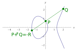
But wait, why -R? We want to find R! Let’s look at the reverse situation, when we are “adding” P and -R points to each other, we get a Q point back, instead of -Q (like 1+(-3) don’t equals 2, but -2). Well, in order to correctly “add” two points we must do second step: negate the received -R point. We only have to draw next line, crossing received point and parallel to the Y axis. This line will cut one more point, which is searched negation.
And what about the points lying on the X axis? From the plot it is clearly visible that such a line will not cut another point. Well, such points are their negation like -0 is also 0 (but note, they are not points alike zero, but more on that later).

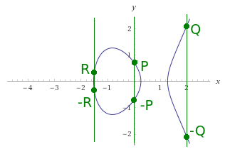
The above plot clearly shows that for the points P, Q, R the rules of addition and subtraction are met by following the described two-step method: P+Q=R, R-Q=P, R-P=Q, -P-Q=-R etc.

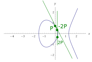
And what about adding one point to itself (eg P+P)? The procedure looks similar, the only difference is the method of determining the first line (we do not have two points, only one). This line must cross this point and be tangent to the plot at this point. Why? Imagine that the selected point has a neighbor on the plot, which is located as close as possible to the selected point (mathematicians would use here the expression ‘+epsilon’, which is the smallest possible, but larger than zero). So we have two points and we can lead the line. Both points on the plot are very, very, very close to each other, so if we enlarge the plot in this place, it will look like the plot between these points is a straight line, so the first line of adding these points “contacts” the plot line.
The tangent line to the plot at the doubled point (P + P = 2P) will cross with one more point, which will be -2P.

And what about (again) the points that lie on the X axis. They also now have to be treated separately because the tangent lines to the plot at these points are parallel to the Y axis, so they will never cross with the plot at another point. If such a line never crosses the plot in another place, it means that it will cut with it at a point in infinity! Well, the elliptical curve has such a special point O, which “is in infinity”. This is the point that is treated with alike zero, so we will also get it by trying to add points P and -P to each other. It can not be marked on the plot, but you can add another point to it, and the result will be added point (O + P = P because the point O is alike zero).

Drawing plot intuitive, but impractical and inaccurate. Therefore, all the above actions on points of the elliptical curve can be written with formulas.

Addition of two points P+Q = R, where:

$P\neq Q$
$P\neq -Q$
$P=\left (x_{p}, y_{p}\right )$ , $Q=\left (x_{q}, y_{q}\right )$ , $R=\left (x_{r}, y_{r}\right )$

looks as follows:

$s=\frac{y_p-y_q}{x_p-x_q}$
$x_r=s ^2 - x_p - x_q$
$y_r=-y_p+s\left( x_p-x_r\right)$

Doubling the point P + P = 2P = T, where:

$P=\left(x_p,y_p\right)$ , $T=\left(x_t,y_t\right)$
$y_p \neq 0$
$y^2=x^3+ax+b$

looks as follows:

$s=\frac{{3x_{{p}}}^{2} + a}{2y_p}$
$x_t=s^2-2x_p$
$y_t=-y_p+s\left(x_p-x_t\right)$

In addition, special cases:
Doubling the point $P=\left(x_p,y_p\right)$ , where $y_p=0$ : P+P=O
Adding negation P+(- P)=O
Adding a point in infinity: P+O=P

This is the end of the high school level theory. The above formulas are easy for humans, but impractical for a computer because they use real numbers. Let’s look at the previously used number $\frac{\sqrt{2}}{2}$ , which is approximately 0.7071067811865476… The computer mainly uses fixed-point numbers but can simulate real numbers using floating-point numbers, which, however, can only be approximations of numbers that can have infinitely many decimal places (floating point type ‘float’ can store something like a dozen or type ‘double’ dozens of decimal places). However, such inaccuracy is unacceptable from the point of view of cryptography, therefore the above elliptical curves of real numbers are not used in IT.

The next part will show what curves and how they are used in digital cryptographic protocols.

Go to part two

Month: June 2018

Elliptic curves and how to use them (part one)