Go to part two
Modern popular processors are able to accurately and efficiently handle integer operations. Therefore, when implementing actions on elliptic curves, it is worth using this property. The type of elliptic curve that is best suited for use in a software solution will be discussed below.
Let’s choose a certain number p, which is a prime number. The bigger this number is the better safety will be assured. For ease of understanding, I suggest choosing number 7 for our next examples.
Let’s create an algebraic structure consisting of a set of numbers {0, p-1} and an operation  such that for a b = (a + b) modulo p. We see that the operation is well defined – modulo p always returns an unequivocal result in the range {0, p-1}. Let’s check now whether this structure is a group. Operation is associative:
(a b) c = ((a b) + c) modulo p = (((a + b) modulo p) + c) modulo p = (a + b + c) modulo p = (a + ((b + c) modulo p)) modulo p = (a + (b c)) modulo p = a (b c).
The neutral element (as in the normal addition) is 0:
0 a = (0 + a) modulo p = (a) modulo p = a
Every element have got also an inverse element:
 = (a + (p – a)) modulo p = (p) modulo = 0
The operation is also commutative:
a b = (a + b) modulo p = (b + a) modulo p = b a
So the structure ({0, p-1}, ) is an abelian group.
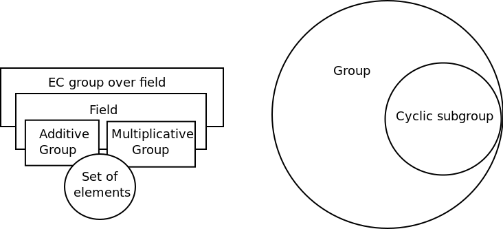
Let’s add the second operation  (a b = (a * b) modulo p) to this structure and see if the structure is a field. The first of the three conditions is met above (({0, p-1}, ) is a group). Let’s check if ({1, p-1}, ) is also a group.
The operation is associative, which can be proved exactly as for .
The neutral element (as in normal multiplication) is 1:
1 a = (1 * a) modulo p = (a) modulo p = a
Every element have got also an inverse element:
1 =  = (
= ( ) modulo p, so from modulo we have = l * p + 1 – it’s linear diophantine equation , so it has a solution because GCD(a, p) = 1 (greatest common divisor).
The operation is also commutative:
a b = (a * b) modulo p = (b * a) modulo p = b a
So the structure ({1, p-1}, ) is also an abelian group.
The last requirement is that operation should be distributive over : (a b) c = ((a + b) modulo p) c = ((a + b) * c) modulo p = (a * c + b * c) modulo p = (a * c modulo p) (b * c modulo p) = a c b c
So we can conclude that the structure Fp = ({0, p-1}, , ) is a field.
The inverse element of operation can be calculated using the diophantic equation, but it is easier to do so using the modified Euclid’s algorithm to calculate the GCD between a and p:
#!/usr/bin/python

def invers(a, p):
    #this only work when p is prime!
    i = p
    j = a
    y2 = 0
    y1 = 1
    while(j > 0):
        q = i/j
        r = i - (j * q)
        y = y2 - (y1 * q)
        i = j
        j = r
        y2 = y1
        y1 = y
    return (y2 % p)
A simple implementation of operations in the Fp field could look like below:
#!/usr/bin/python

...

class FieldElement:
    def __init__(self, p, value):
        if(value >= p):
            raise ValueError('value %s outside field (p=%s)'%(value, p))
        self.p = p
        self.value = value

    def __str__(self):
        if self.value < 0:
            return "-0x%x"%(self.value*(-1))
        return "0x%x"%self.value

    def __add__(self, other):
        if type(other) == int or type(other) == long:
            return FieldElement(self.p, ((self.value + other) % self.p) )
        else:
            return FieldElement(self.p, ((self.value + other.value) % self.p) )

    def __sub__(self, other):
        if type(other) == int or type(other) == long:
            return FieldElement(self.p, ((self.value - other) % self.p) )
        else:
            return FieldElement(self.p, ((self.value - other.value) % self.p) )

    def __mul__(self, other):
        if type(other) == int or type(other) == long:
            return FieldElement(self.p, ((self.value * other) % self.p) )
        else:
            return FieldElement(self.p, ((self.value * other.value) % self.p) )

    def __truediv__(self, other):
        if type(other) == int or type(other) == long:
            inv = invers(other, self.p)
        else:
            inv = invers(other.value, self.p)
        return FieldElement(self.p, ((self.value * inv) % self.p) )

    def __eq__(self, other):
        return (self.value == other.value)

    def __ne__(self, other):
        return (self.value != other.value)

    @staticmethod
    def factoryMethod(otherFieldElement, value):
        return FieldElement(otherFieldElement.p, value % otherFieldElement.p)
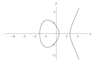
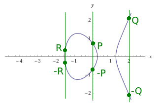
Let’s see how we can use the Fp field to create elliptic curves. At first glance, the EC formula looks identical:

however, in this case we have used elements and operations from the field Fp instead of the field of real numbers. The curve here must meet an additional condition: (4 *  + 27 *
  ) modulo p = 0.
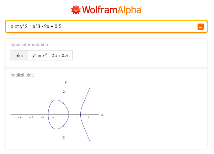
The curves above the Fp fields are less intuitive than the curves above the R body, as shown in the following graphs:
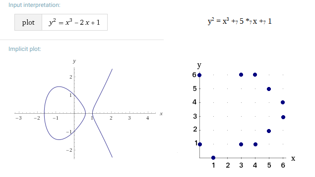
In general, the points of the EC(Fp) curve appear to be “randomly” arranged with some symmetry. Points do not lie at every x position. Usually there are two points on one x position excluding points whose position y = 0 (in the example above it is point (1, 0), which, however, is in symmetry with itself – theoretically it is also point (1,7)).
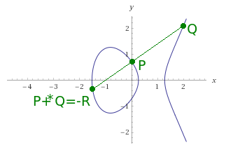
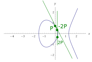
The operations on the EC(Fp) curve look quite identical to those on the EC(R) curve with the difference that + * opeations are replaced by and .
And so point negation looks like (the only major difference):
(mod%20%5C%3Bp)))
Adding two points ( ,
,  ,
,  ):
):
%5Cast(x_a-x_b)%5E%7B-1%7D%5C%3B%5C%3B%5C%3B(mod%20p))
)
%5C%3B%5C%3B%5C%3B(mod%20p))
Doubling the point ( ,
,  ):
):
%7B%5Cast%7D(2y_a)%5E%7B-1%7D%5C%3B%5C%3B%5C%3B(mod%20p))
))
%5C%3B%5C%3B%5C%3B(mod%20p))
Special cases are also identical:
Doubling ) gives neutral point (point in infinity).
gives neutral point (point in infinity).
Adding negation ) gives neutral point.
gives neutral point.
Adding  to neutral point gives point .
The last needed element of EC(Fp) arithmetic is point multiple. Most often it is called point multiplication, but this operation is more understood here as exponentiation in the additive group version.
Traditional exponentiation is the number of multiplications of a given number that we must do to obtain the result of exponentiation. And so if we have  then we must multiply the number three four times: 3 * 3 * 3 * 3 = 81. But what if we have to calculate
  ? Of course, we can do 3 * 3 * … * 3 – 112 multiplications (and each multiplication operation costs some computational power), or write as
 %20%5E%202%20)%20%5E%202)%20%5E%202)%20%5E%202)%20%5E%202) , where we have only 9 multiplications.
, where we have only 9 multiplications.
And so, if we have a certain point on EC and want to multiply it by 117, then instead of 116 additions, we can write this number to binary form 1110101 and moving from the least significant bit follow the steps of a simple algorithm:
- For the start the base point B equals the multiplied point P, and the ‘result’ point R equals the neutral point.
- If the considered bit is one, add point B to point R.
- If this is not the last bit, double the B point and go to step 2 considering the next bit.
The result of the algorithm is point R. In our example for 117 * P, the algorithm will perform only 5 additions and 6 doubles.
Using the previous Fp implementation, we can now also implement EC(Fp) arithmetic:
#!/usr/bin/python

import copy

...

class ECPoint:
    def __init__(self, p, a, b):
        testec = (4*a*a*a) + (27*b*b)
        if(testec %p == 0):
            raise ValueError('Bad EC')
        self.a = FieldElement(p, a)
        self.b = FieldElement(p, b)
        self.neutral = True

    def __str__(self):
        if self.neutral:
            return "(neutral)"
        return "(0x%x,0x%x)"%(self.x.value, self.y.value)

    @staticmethod
    def testOnCurve(a, b, x, y):
        test_left = y*y
        test_right = x*x*x+a*x + b
        if test_left.value == test_right.value:
            return True
        return False

    def testOnSelfCurve(self):
        if self.neutral:
            return True
        return ECPoint.testOnCurve(self.a, self.b, self.x, self.y)

    @staticmethod
    def factoryMethod(otherECPoint, x, y):
        if not ECPoint.testOnCurve(otherECPoint.a, otherECPoint.b, x, y):
            raise ValueError('Point not on EC')
        res = copy.deepcopy(otherECPoint)
        res.x = x
        res.y = y
        res.neutral = False
        return res

    def double(self):
        if self.y.value == 0:
            return ECPoint(self.a.p, self.a.value, self.b.value) #return neutral
        s1 = (self.x*self.x*3) + self.a
        s2 = self.y*2
        s2 = invers(s2.value, s2.p)
        s = s1*s2


        x = (s*s) - (self.x*2)
        y = s*(self.x - x) - self.y
        return ECPoint.factoryMethod(self, x, y)

    def __add__(self, other):
        if self.neutral:
            return copy.deepcopy(other)
        elif other.neutral:
            return copy.deepcopy(self)
        elif other.x == self.x and other.y == self.y:
            return self.double()

        s1 = self.y - other.y
        s2 = self.x - other.x
        s2 = invers(s2.value, s2.p)
        s = s1*s2

        x = s*s - self.x - other.x
        y = s*(self.x - x) - self.y
        return ECPoint.factoryMethod(self, x, y)

    def __mul__(self, other):
        if type(other) == FieldElement:
            other = other.value
        elif type(other) != int and type(other) != long:
            raise ValueError("Can't multiply by %s"%(type(other)))

        res = ECPoint(self.a.p, self.a.value, self.b.value) #start with neutral
        base = copy.deepcopy(self)
        mask = 1
        while True:
            if mask & other:
                res += base
            mask <<= 1
            if mask > other:
                break
            base += base
        return res
We must be sure that the implementation we created is correct. The easiest way to verify it is to select a point and perform some operation on it (e.g. doubling it, then adding it to the doubling result) – the obtained point should be a point that also lies on the curve (satisfies the curve equation). This is a test to verify basic errors, but it is not enough.
The main verification tool are test vectors. For example, in the document rfc5903 in section 8.1 we have a test vector for a 256 bit curve (from section 3.1). if we take the point ‘g’ (from 3.1) and multiply it by ‘i’ (from 8.1), we should get ‘gix’ and ‘giy’ values:
#!/usr/bin/python

...

p = (2**256)-(2**224)+(2**192)+(2**96)-1
tv = FieldElement(p, 1)

neutral = ECPoint(p, -3, 0x5AC635D8AA3A93E7B3EBBD55769886BC651D06B0CC53B0F63BCE3C3E27D2604B)

gx = FieldElement.factoryMethod(tv, 0x6B17D1F2E12C4247F8BCE6E563A440F277037D812DEB33A0F4A13945D898C296)
gy = FieldElement.factoryMethod(tv, 0x4FE342E2FE1A7F9B8EE7EB4A7C0F9E162BCE33576B315ECECBB6406837BF51F5)

g = ECPoint.factoryMethod(neutral, gx, gy)

i = 0xC88F01F510D9AC3F70A292DAA2316DE544E9AAB8AFE84049C62A9C57862D1433
r = 0xC6EF9C5D78AE012A011164ACB397CE2088685D8F06BF9BE0B283AB46476BEE53
gi = g*i
gr = g*r
print "gi(%s)=%s"%(gi.testOnSelfCurve(), gi)
print "gr(%s)=%s"%(gr.testOnSelfCurve(), gr)
gir = gi*r
gri = gr*i
print "gir(%s)=%s"%(gir.testOnSelfCurve(), gir)
print "gri(%s)=%s"%(gri.testOnSelfCurve(), gri)
gi(True)=(0xdad0b65394221cf9b051e1feca5787d098dfe637fc90b9ef945d0c3772581180,0x5271a0461cdb8252d61f1c456fa3e59ab1f45b33accf5f58389e0577b8990bb3)
gr(True)=(0xd12dfb5289c8d4f81208b70270398c342296970a0bccb74c736fc7554494bf63,0x56fbf3ca366cc23e8157854c13c58d6aac23f046ada30f8353e74f33039872ab)
gir(True)=(0xd6840f6b42f6edafd13116e0e12565202fef8e9ece7dce03812464d04b9442de,0x522bde0af0d8585b8def9c183b5ae38f50235206a8674ecb5d98edb20eb153a2)
gri(True)=(0xd6840f6b42f6edafd13116e0e12565202fef8e9ece7dce03812464d04b9442de,0x522bde0af0d8585b8def9c183b5ae38f50235206a8674ecb5d98edb20eb153a2)
And we quickly proved that the presented implementation is correct.
In the next part we will deal with the optimization of this curve arithmetic implementation.
ec_part3 (full code)
go to part 4
,