Elliptic curves and how to use them (part two)

Go to part one

There should be presented a bit simplistic theory from the so-called “algebraic structures” before showing method of implementing elliptic curves on digital devices.
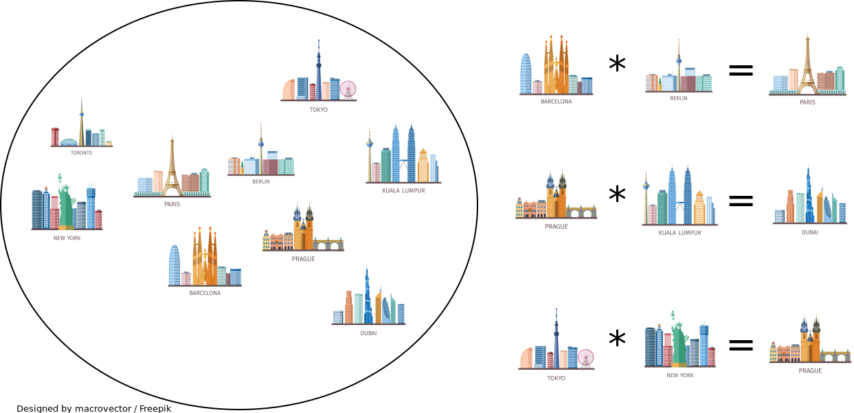
So what is this algebraic structure? This is a non-empty set with at least one operation in this set: $S= \{ A, \ast_{1}, \ast_{2}, ... \}$ . What can contain such a set? Numbers, colors, cities etc: $A= \{ a_{1}, a_{2}, a_{3}, ...} \}$ . What can this operation be like? Addition, multiplication, but also returning a city lying between two selected cities: $\ast_{i}: a_{x} \times a_{y} \rightarrow a_{z}$ .

For the needs of EC, we will consider structures with finite sets with two-arguments operation or two two-arguments operations: $S= \{ A, \ast \}$ or $S= \{ A, \ast_{1}, \ast_{2} \}$ .

If the structure $S= \{ A, \ast \}$ meets the following requirements:

operation $\ast$ is associative: $a_{1} \ast a_{2}\) \ast a_{3} = a_{1} \ast \( a_{2} \ast a_{3}$
set A has a identity element e for operation $\ast$ : $a_{i} \ast e = e \ast a_{i} = a_{i}$
each element $a_{i}$ from set A have it’s inverse element $a_{j}$ : $a_{i} \ast a_{j} = a_{j} * a_{i} = e$

we can call this kind of algebraic structure a group.
Additionally, if the $\ast$ operation is commutative for each $a_{i}, a_{j}$ : $a_{i} \ast a_{j} = a_{j} * a_{i}$ , then this group is called an commutative or abelian group.

There are two ways of group’s write:

additive: G = {A, +}, where the identity element is presented as ‘0’ and the inverse element of a as -a (like in ‘traditional’ adding)
multiplicative: G = {A, $\ast$ }, where the identity element is presented as ‘1’, and the inverse element of a as $a ^{-1}$ (like in ‘traditional’ multiplication).

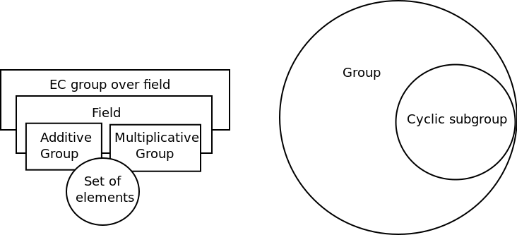
If element A which is not a identity element is selected from the set A, which will be used to the following operations: $a_{g} \ast a_{g} = a_{1}, a_{g} \ast a_{1} = a_{2}, a_{g} \ast a_{2} = a_{3}, ..., a_{g} \ast a_{n} = e$ , it creates a subset $H = \{e, a_{g}, a_{1}, a_{2}, a_{3}, ..., a_{n} \}$ ( $H\subseteq G$ – H is subset of G) which with $\ast$ operation is a subgroup that is called a cyclic group, and $a_g$ is a generator of this group. The set H can be also two-element $\{e, a_g\}$ , and exactly a set G (H = G). So the whole group G is a cyclic group, if there is at least one element $a_g \in G$ , from which any other element of the group can be created: $a_i = i \ast a_g$ (additive write) or $a_i = a_g^i$ (multiplicative write).
If a set of all points lying on a certain elliptical curve is taken and as a set EC and addition of two of these points will be marked as + operation (described in the previous section), then G = {EC, +} is an abelian group. A point g is also selected for creating a cyclic sub-group H = {ECH, +}.
And that’s all to show how elliptic curves work as a theory, however, this is not enough yet to show the way the EC is implemented.

If the structure $S=\{A, \ast_1, \ast_2\}$ meets the following requirements:

structure $S_1=\{A, \ast_1\}$ is an abelian group (commutative)
structure $S_2=\{A/ \{0\}, \ast_2\}$ (without a identity element of group $S_1$ ) is also an abelian group (commutative)
operation $\ast_2$ is distributive over $\ast_1$ : $(a_i \ast_1 a_j) \ast_2 a_k = (a_i \ast_2 a_k)\ast_1(a_j\ast_2 a_k)$ and $a_i \ast_2 (a_j \ast_1 a_k) = (a_i \ast_2 a_j)\ast_1(a_i\ast_2 a_k)$

this is the structure we call the field and, for simplicity, we write K = {A, +, $\ast$ }.

Let’s now look back at the EC chart from the previous section:

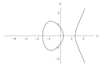
The graph consists of two X, Y coordinates on which the real numbers are located. Real numbers can be added and multiplied. If an algebraic structure consisting of an infinite set of real numbers, additions and multiplication is constructed, it will turn out that such a structure is a field. Thus, it can be seen that the EC lies on a dimensional space over field.

We know that the field of real numbers is not suitable for implementation on digital devices due to its infinite number of elements and the need for infinite accuracy of calculations. So what field can we use? It turns out that there are two types of finite fields that are ideally suited for the software and hardware implementation. In the nearest parts, we will deal with fields for software implementation.

Go to part three

Post Views: 35

Leave a Reply Cancel reply